Recommendation Systems - Brief overview of Matrix Factorization
The User-Item Matrix:
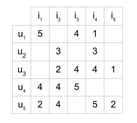
Suppose we had a user-item matrix like the one below, where each cell represents what a given user (u) has rated an item (i).

There are several missing entries in this matrix, which represent the ratings that we want to predict, and eventually recommend to the user. If you were working at Netflix, these ratings could mean the number of stars a user has rated a given movie.
Matrix Factorization:
One way of performing collaborative filtering is via matrix factorization. In matrix factorization, we try to find two low rank matrices U and V, such that when multiplied together, they recreate the original sparse matrix.

- The dimensions of the user matrix U is u x d, whether u is the total number of users and d is the number of hidden features.
- The dimensions of the item matrix I is d x i, where, again, d is the number of hidden features, and i is the total number of items
These d hidden features represent the hidden attributes for a given user or item, which capture the essence for that given user or item. For example a given user might have hidden features which represent the degree they like action movies, or the degree they like Disney movies, or their preference for a female or male lead actor. When a uxd user-factor matrix is multiplied by a dxi item factor matrix, it will create the original uxi user-item matrix with the predicted ratings for the missing values.
Matrix Factorization with Singular Value Decomposition:
We can use a technique such as Singular Value Decomposition (SVD) to decompose the matrix into:
, the user factor matrix consisting of m users and k hidden features.
, a diagonal matrix which contains the k singular values of the original matrix
, the item factor matrix, consisting of n items and k hidden features.
One disadvantage of using SVD it that is an analytical approach for decomposing the matrix, requiring that all the values in the matrix to be filled with some value before the SVD can be performed.
When the matrix becomes too sparse (say less than 1% of the entries of the matrix are filled), then it becomes very difficult to infer these empty items using a traditional SVD. You can try imputing missing values with the mean of median of a row or column, but this would lead to biased results. In this case, your SVD would be biased towards computing the mean or median values that you imputed the matrix with.
Matrix Factorization using a Machine Learning Based Approach (ALS):
Alternatively, we can use a machine-learning based approach to learn the user-factor and item-factor matrices.
Essentially, the goal here is the same as an SVD, we want to learn the two low rank user-factor and item-factor matrices such that when multiplied together, they reconstruct the original sparse user-item matrix.
The objective function we are trying to minimize is the following:
Essentially, we are trying to minimize the difference between
Taking the derivative of the cost function with respect to the user-factor matrix x, we can solve for x and get the following:
Similarly, taking the derivative of the cost function with respect to the item-factor y matrix, we can solve for y and get the following:
Now that we have these derivatives computed, the ALS algorithm goes as follows:
1. Initialize the user-factor matrix x and item factor y with random numbers.
2. Fixing y, update the user-factor matrix x using the first formula
3. Fixing x, update the item-factor matrix y using the second formula
4. As you keep iterating on steps 2 and 3, the total loss will decrease. Keep iterating until convergence.
A numpy implementation can be found here:
Additional Resources:
- http://yifanhu.net/PUB/cf.pdf
- http://ethen8181.github.io/machine-learning/recsys/1_ALSWR.html
- https://datasciencemadesimpler.wordpress.com/tag/alternating-least-squares


Cool stuff!!!
ReplyDelete